Genetics, meiosis
Study Questions:
1. What are the five assumptions of the Hardy-Weinberg Equilibrium Model?
2. Consider the following population:
| AA | Aa | aa | |
|---|---|---|---|
| Number of Individuals | 60 |
20 |
20 |
and some lecture notes you might find helpful...
II. Transition to Post-Darwinian Theory: Population Genetics
A. Introduction
- As you see below, evolution is now defined as a "change in the genetic structure of a population". Population genetics studies how these genetic changes occur in populations. You see, organisms can only live, reproduce, and die; individual organisms do NOT evolve (they develop). Evolution is the change that occurs over time in a group of organisms - a population. So, we need a way to describe the genetic changes occuring at this scale of biological resolution (not the individual but the population...)
1. DEFINITIONS
- Evolution: a change in the genetic structure of a population
- Population: a group of interbreeding organisms that share a common gene pool;
spatiotemporally and genetically defined
- Gene Pool: sum total of alleles held by individuals in a population
- Genetic structure: Gene frequencies and Genotypic Frequencies
- Gene/Allele Frequency: % of alleles at a locus of a particular type
- Gene Array: % of all alleles at a locus: must sum to 1.
- Genotypic Frequency: % of individuals with a particular genotype
- Genotypic Array: % of all genotypes for loci considered; must = 1.
2. BASIC COMPUTATIONS
a. Determining the Genotypic and Gene Arrays
AA
Aa
aa
Number of Individ. (observed)
25
40
35 (100)
Genotypic Array
25/100=.25 40/100=.4
35/100=.35 = 1.00
Number of A alleles
50
40
0 = 90/200=.45
Number of a alleles
0
40
70 =110/200=.55
Gene Array = .45(A) + .55(a) = 1.00
b. Short Cut Method: Determining the Gene Array from the Genotypic Array
a. f(A) = p = f(AA) + f(Aa)/2 = .25 + .4/2 = .25 + .2 = .45
b. f(a) = q = f(aa) + f(Aa)/2 = .35 + .4/2 = .35 + .2 = .55
3. KEY: The Gene Array CAN ALWAYS be computed from the genotypic
array; the process just counts alleles instead of genotypes.
B. The Hardy-Weinberg Equilibrium Model
1. GOALS
a. Objective: Determine whether evolution is occuring, and if so, identify the
cause
b. Basic Method: Predict what the genotypic array would be if genes were
distributed randomly and there is NO CHANGE (create an expected model).
Then, see how the real population differ from this model.
c. Hardy and Weinberg realized that, in order for probability to be explicitly
TRUE in describing the genetic structure of the population, the we must assume
that the population is infinitely large (so there is no chance of radom "sampling"
error). Also, in order for there to be NO CHANGE, then these additional
conditions must be met:
- random mating (so gametes come together probabilistically)
- no selection (all organisms survive and pass on their genes a the same rate)
- no mutation ("A's" can't be changing into "a's" behind our back...)
- no migration (there can't be organisms bringing in their genes into our population)
d. Hardy and Weinberg demonstrated that, if these conditions were met, there would be NO SUBSEQUENT CHANGE - NO EVOLUTION. So, we can use this model for comparison, as a theoretical expectation, to see if a real population is conforming to these expectations (and is NOT evolving), or differs from these expectations of the model (and therefore IS evolving).
2. EXAMPLE:
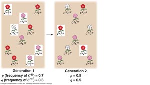
- Consider a population with the following genetic structure:
AA Aa aa
Genotypic Frequencies:
0.6 0.2 0.2
So, the gene frequencies are: A = 0.6 + (0.2/2) = 0.7
a = 0.2 + (0.2/2) = 0.3
Now, consider this gene pool in which 70% of the alleles are 'A' and 30% of the alleles are 'a'.
IF THE POPULATION MATES RANDOMLY, THEN::
The probability of an 'A' egg meeting an 'A' sperm is (0.7)*(0.7) = p2
= 0.49
So, you would expect the frequency of AA zygotes in the next generation to be
0.49
The probability of an 'a' egg meeting an 'a' sperm is (0.3)*(0.3) = q2
= 0.09
So, the frequency of these zygotes is 0.16
Aa zygotes can be formed two ways; 'A' sperm meets 'a' egg (0.7)*(0.3) = 0.21
and 'a' sperm meets 'A' egg (0.3)*(0.7) = 0.21. So, the total probability
= 2pq = 0.42
So, if the population mates RANDOMLY,
THEN thethe Genotypic Array should be: AA Aa aa
0.49 0.42 0.09
Well, sort of. ACTUALLY, we would only be ABOLUTELY SURE that these would be the genotypic frequencies IF:
- nothing had changed the gene frequencies (there is no mutation changing one gene into another, no migration "bringing in" A's from another place, and no selection in which A's are "better" than a's so they survive longer in teh gene pool and mate more often).... so there can be NO MUTATION, MIGRATION, OR SELECTION.
- Also, in order for us to be PERFECTLY SURE that the population will produce THESE geneotypic frequencies EXACTLY, with no sampling error, the population must be INFINITELY LARGE.
- So, If there is random mating and no mutation, migration, or selection in a n infinitely large population, these genotypic frequencies should be produced in the offspring. Tomorrow we will see why this is an EQUILIBRIUM, and we will examine why this is such a useful model for evolutionary theory.
3. UTILITY
- If no real populations can explicitly meet these assumptions, how can the model be useful? For instance, no real population is infinitely large...
- We use it for COMPARISON. This model describes what the genotypic frequencies
should be IF the population was in equilibrium. If the real genotypic
frequencies are not close to these expectations, then:
- the population is not in HWE.... it is evolving.
- and if it IS NOT in HWE, then one of the assumptions must be violated.
Think about that. The HWE is only 'true' if the assumptions are being
met. If your real population differs from the model, then one of the assumptions
must not apply to your real population. This narrows your focus on WHY
the real populations isn't behaving randomly... and it might identify WHY the
population is evolving.
- In class, we used the coin analogy. No REAL coin is probably exactly perfectly balanced. But, if I give you a coin and ask you how balanced it is, you flip it a few times and compare its behavior to WHAT YOU WOULD EXPECT FROM A PERFECT COIN (50:50 RATIO). Even though a perfectly balanced coin does not exist, we can use this theoretical model as a benchmark, to compare the behavior of real coins. Many real coins act in a manner that is consistent enough with the expectations from a perfectly balanced coin that we are willing to use them AS IF they were perfectly balanced.
- Hardy Weinberg Equilibrium Model is the same... it is a model of no change against which we can measure real populations. Why would real populations differ from this model? BECAUSE THEY VIOLATE ONE OR MORE OF THE ASSUMPTIONS!! Know this logic.
Example:
Suppose you observe the following number of individuals in a real population:
AA Aa aa Number of Individuals You'd calculate the gene frequencies as p = 0.6 and q = 0.4.
The genotypic FREQUENCIES, and the number of individuals you'd expect to see in a population of 200, would beyou'd EXPECT to see if the population was in HWE would be:
AA Aa aa Number of Individuals HWE EXPECTED FREQ's(p^2, 2pq, q^2) HWE expected number (out of 200) Now, we use a goodness-of-fit test to compare our observed and expected values.
Our critical value from the table, with df = 2 and p = 0.05, = 5.99.....
Obviously we are way over, so we reject the hypothesis on which our expected values are based. We reject the hypothesis that this population is in HWE. So, if it's NOT in equilibrium, it must be changing... and a changing population is EVOLVING.